磨刀不误砍柴工 系列之 三 : Dynamic Programming

August 06, 2014

Dynamic Programming (DP) is a general algorithm design paradigm. Its inventor is Richard Bellman. DP is originated from his mathemetical research.

DP is really difficult to understand. Cause it’s not a concrete algorithm pattern. It depends more on the aiming problem.

Then I will study DP case by case at first. It seems more convenient and easier to be understood.

The materials I have referenced also includes MIT Algorithm Open Course:
19. Dynamic Programming I: Fibonacci, Shortest Paths
20. Dynamic Programming II: Text Justification, Blackjack
21. Dynamic Programming III: Parenthesization, Edit Distance, Knapsack

A well-known guide from TopCoder: Dynamic Programming: From novice to advanced

Fibonacci Number

We define Fibonacci Number algorithm as following:

F(1) = F(2) = 1
F(n) = F(n-1) + F(n-2)

\(\because T(n) = T(n-1) + T(n-2) + \Theta(1) \geq 2T(n-2) = \Theta(2^{n/2})\)
\(\therefore \)The traditional recursive algorithm has a time complexity of \(\Theta(2^{n/2})\).

In order to calaulate F(n), you have to calculate F(n-1) and F(n-2) first; in the same way, you should calculate F(n-2) + F(n-3) –> F(n-1), F(n-3) + F(n-4) –> F(n-2) . So, there will be some duplicated calculation during the recursion. Such as you have to calculate F(n-3) twice.

But in DP, a Buttom-up DP algorithm could avoid the duplication.

fib= {} // used to memorize the calculated Fibonacci Number
for k in range[1, n+1]
    if k <= 2: f = 1
    else: f = fib[k-1] + fib[k-2]
    fib[k] = f
return fib[n]

So, the order of complexity comes down to \(O(n)\).

A more detailed guide for Fibonacci Number in DP, see: Fibonacci series and Dynamic programming.

0-1 Knapsack Problem

We shall first introduce the Fraction Knapsack Problem (FKP). This is, we are allowed to take fractional amounts.

For example, in Figure 1 there are several bottles of milk to choose, the volume and value per ml are different. We could choose 10ml at most among those bottles.

The strategy is simple. We could simply choose from with the highest value milk greedly.

Figure 1: Fraction Knapsack Problem

But in 0-1 Knapsack Problem (0-1KP), we cannot divide the choices fractionally.
For a simple separated example, if we can still take only 10ml milk. But the choices are 2ml/8value, and 9ml/9value.
In FKP, we can take the total 2ml/8value, and then partially 8ml/8value from 9ml/9value.
But in 0-1KP, we cannot divide the 9ml/9value milk partially. So we have to take only 9ml/9value in order to maximum the benefit.

The stratedy is clear. But the algorithm is a little difficult to be understood. Here is the pseudo-code:

Algorithm 01Knapsack(S, W):
  Input: set S of n items with benefit b_i and weight w_i; maximum weight W
  Output: benefit of best subset of S with weight at most W
  let A and B be arrays of length W + 1
  for w <-- 0 to W do
  B[w] <-- 0
  for k <-- 1 to n do
    copy array B into array A
    for w <-- w_k to W do
      if A[w - w_k] + b_k > A[w] then
        B[w] <-- A[w - w_k] + b_k
  return B[W]

The difficult lines are 9 ~ 11. What I have now realized is:

• The size of B[w] is actually equals W+1;
• A new item k will be tested from 0 to W - w_k, no matter that it is valuable to be inserted or not,
  This means, B[w] will only be scaned & updated from w_k to W.
• And the set B[w] will only be changed partially; not necessarily successive changes, either.
  eg: Assume the size of Figure 2 is 12, and (3,2)(5,4)(8,5) are in position, where (value,volumn) is one pair. So, B[w] = {0,0,3,3,5,8,8,11,11,13,13,16}.
  If a (2,1) is coming, then B[w] = {0,2,3,5,5,8,8,11,13,13,15,16}; there is no change for the final result B[W] (here is B[12])
  Unless there is another (2,1) is coming, then B[w] = {0,2,4,5,7,8,10,11,13,15,15,17}. Thus the updated result of B[W], which is B[12] in this case, is changed from (3+5+8) to (2+2+5+8).

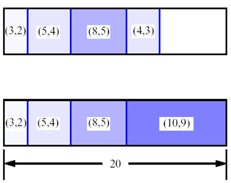Figure 2: 0-1 Knapsack Problem

Although this examination verified the algorithm is true, there is still far away from understanding the algorithm by reasoning it logically. But the examination with real data at least reavels some features of this algorithm:

• This algorithm’s running time structure is more complicated than I had thought of it;
• Everytime a new item is inserted, the changing of the original B[w] is insuccessive. But It ensures recoding the extra information of the new input, whether the final B[W] will be changed or not;
• The size of the set is B[W+1] instead of B[W].

(Another version of pseudo-code gets rid of the assistent array A[w], it replaces lines 8~11 with the following:

for w <-- W downto w_k do
    if B[w - w_k] + b_k > B[w] then
        B[w] <-- B[w - w_k] + b_k

I have examed this version. It showed the same B[w] structure as the previous one in the runing time.)

Last but not least, in NP-Completeness theorem, the KNAPSACK optimization problem has a fully polynomial approximation scheme that achieves a \( (1+\varepsilon) \)-approximation factor in \( n^3/\varepsilon \) time, where \( n \) is the number of items in the KNAPSACK instance and \( 0 < \varepsilon < 1 \) is a given fixed constant.

Shortest Path

Matrix Chain-Product

The one, most confused one to me among aboving.

DP的另一种思路 与 不变的共同点

DP不是一种具体的算法，可能会有雷同的题用雷同的解法，但不应该有思路上的限制。

我的DP思路一直受限于 0-1 Knapsack Problem 上，下面这题在算法的结构上算是另一种相反思路：

上面这题其实不是一个用DP解决的问题，是利用DFS的Recursion来解决的。

但是DP的思路灵活却是一句实话。看这个例子：

Longest Monotonically Increasing Subsequence Size (N log N)

static int lisLength(int[] A) {
  // Add boundary case, when array size is one
  int[] tailTable = new int[A.length];
  int len; // always points empty slot

  tailTable[0] = 0;
  len = 1;
  for (int i = 1; i < A.length; i++) {
    if (A[i] < tailTable[0]) {
      // new smallest value
      tailTable[0] = A[i];
    }
    else if (A[i] > tailTable[len - 1]) {
      tailTable[len++] = A[i]; // Because len always points empty slot, so use len++ rather than ++len
    }
    else {
      // A[i] wants to be current end candidate of an existing subsequence
      // It will replace ceil value in tailTable
      tailTable[ceilIndex(tailTable, -1, len - 1, A[i])] = A[i];
    }
  } // end of for
  return len;
}

// Binary search (note boundaries in the caller)
// A[] is ceilIndex in the caller
static int ceilIndex(int[] A, int l, int r, int key) {
  int m = 0;
  while (l < r - 1) {
    m = (l + r) / 2;
    if (A[m] >= key) {
      r = m;
    } else {
      l = m;
    }
  }
  return r;
}

思路和0-1 Knapsack很不相同，但他们都有一个共同点，就是用状态转移方程把一个大问题变成几个小问题，甚至在很多情况下有递推的效果，类似数学中的__归纳证明法__。

List of DP Problems

罗列了一些我见过的DP问题，仅仅只是用DP做cache加速的问题(比如Fibonacci)就不列举了。

令，DP问题中，关键在于寻找状态转移方程 (TopCoder那篇原文并没有提到过这个term)；用DP做cache加速的问题中，这个方程可以叫做优化方程 Optimal Function

1. Maximum sell stock profit within given days

2. 自行搜索此列表中的DP关键字: leetcode难度及面试频率

References

TopCoder上一篇著名的DP文章 Dynamic Programming: From novice to advanced 中文翻译版 动态规划：从新手到专家]

DP问题各种模型的状态转移方程