Spam Filter (2) -- Bayes Theorem & Graham's Method

January 27, 2014

The basic algorithm of my Bayesian Filter is studied from Paul Graham’s post A PLAN FOR SPAM. I was firstly attracted on this topic by a Chinese version of it: 贝叶斯推断及其互联网应用: 定理简介 和 过滤垃圾邮件 (2011) Ruan Yi-feng (Bayesian Inference and Web Application: Introduction to the Theory & Spam Filtering)

I also made some improvement based on it to access higher AUC.

Basic Theory

Given an unlabeled mail, I can calculate the probability of how much it will be a Spam. \[ P = \frac{P(S|W1) \ast P(S|W2) \ast P(S)}{P(S|W1) \ast P(S|W1) \ast P(S) + (1 - P(S|W1)) \ast (1 - P(S|W2)) \ast (1 - P(S))} \], where \(P(S|Wi)\) is the probability of a mail to be Spam when it contains the word \(Wi\).

Assuming \( P(S) = 0.5 \), then \[ P = \frac{P(S|W1) \ast P(S|W2) }{P(S|W1) \ast P(S|W1) + (1 - P(S|W1)) \ast (1 - P(S|W2)) } \]

In order to calculate \(P\), I just need to know the \(P(S|W)\) value for each Word, which I can learn in training process from the labeled data.
\[ P(S|W) = \frac{P(W|S) \ast P(S) }{P(W|S) \ast P(S) + P(W|H) \ast P(H) } \], where \( P(W|S) \) is the static likelihood of a word existing in all Spam, which I call learned from training data. The same as P(W	H), H is the first Character or Healthy, means Non-spam. I can also assume \(P(S) = P(H) = 50%\) here. (Actually, the provided data also has half number of Spam and half number of Non-spam.)

Implement Graham’s Method

I implemented Graham’s method in four steps.

Step 1. \( P(W|S) \)

Learn the likelihood of each word existing in Spam and Non-spam from train_data or the 1st-half of tune_data; e.g. There are 2000 Spam and 2000 Non-spam in train_data, the number of Spam which has word \(W1\) is 1234, the number of Non-spam which has word \(W1\) is 567. So, \( P(W|S) = 1234/2000 \), \( P(W|H) = 567/2000 \);

Step 2. \( P(S|W) \)

I can now evaluate each mail from u01_eval, u02_eval, or the 2nd-half of tune_data; For each word in a mail, I calculate its \(P(S|W)\), and then I sort all the \(P(S|W)\) of words in this mail by Decreasing order. And I just pick the first some of these words (e.g. 15 words, called interesting words) to calculate the Combining Probability of this mail. This is the probability of this mail to be a Spam.

e.g. \( P = P1P2…P15 / P1P2…P15 + (1-P1)(1-P2)…(1-P15) \), where \(P1\) is the simple symbol of \(P(S|W1)\).

I can predict whether a mail is a Spam or not based on this probability \(P\).

Step 3. Tuning Parameters

There are some parameters not decided yet for evaluation. So the tune_data is used to decide those parameters. I cannot do this tuning process directly on u02_eval because if I did so, I would cheat based on test data. And, I cannot add tune_data into train_data because the word IDs of these two files are different.

Step 4. Optimize Inbox

For u00, I have also a sample of u00_tune_data, which could be used to tune parameters only for u00_eval. With this different parameters, I also train on train_data and then evaluate on u00_eval.

The result of this basic implementation is shown in Table 2:

Table 2: AUC of Basic Implementation of NB

Table1	tune	u01	u02	u00_tune	u00
AUC	0.998056	0.899351	0.951194	0.992355	0.869827
u00_tuned				0.996812	0.894598

The second line in Table 2 is results that evaluated with parameters tuned from file task_a_labeled_tune.tf. The third line is results that evaluated with parameters tuned from file task_a_u00_tune.tf. So this make sense that u00 has its individual features which could be learned separately.

And following Figure 3 is the roc curves in one plot. The red line is a random classifier; the green line of u00 is the curve for result of u00 after parameters tuned from task_a_u00_tune.tf.

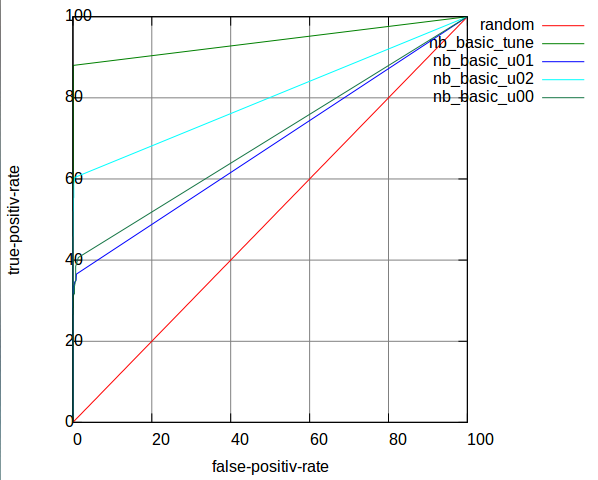
Figure 3: ROC curves of Basic NB

Improve Naive Bayes: Frequency & Anti-Spoof

When I statistic the likelihood, I only +1 time when a word exists in Spam or Non-spam. I have not taken advantage of the frequency information yet.

But if I simply add the true frequency value, it would also not reflect the real likelihood.

e.g. in task_a_labeled_train.tf there is a mail, -1 9:84 35:324 67:2 74:18 92:6 132:3

I think the useful frequency should distinguish the low value, but should not be too big when the value is high. So I hope the frequency can be transformed to something like Figure 4.

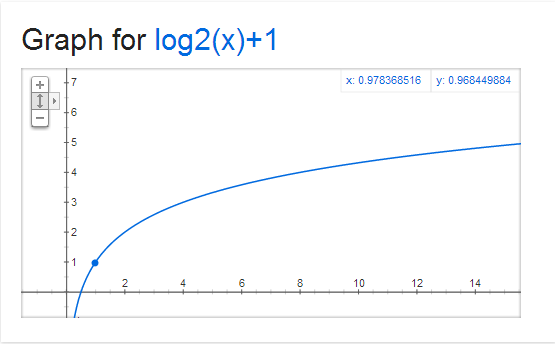
Figure 4: Graph for \( y = log_2⁡x + 1 \)

I choose 2 as the base of the logarithm for the reason that the conversion can distinguish 1 and 2. Here is the relation: 1 -> 1; 2 -> 2; [3,4] -> 3; [5..8] -> 4; etc.

However, there is a problem pointed out by Graham, “such an algorithm would be easy for spammers to spoof: just add a big chunk of random text to counterbalance the spam terms.” (from Better Bayesian Filtering (2003) Paul Graham )

I solve this problem by setting a maximum boundary for transformed frequency. When the transformed value is greater than this boundary, I just omit it for regarding this as a spoofing.

This improvement works, and increases the AUC a bit.

Table 3: AUC of Improved NB

Table1	tune	u01	u02	u00_tune	u00
AUC	0.998196	0.912002	0.952196	0.991569	0.874134
u00_tuned				0.991257	0.901313

I lost the parameters here, actually I can get 1% higher AUC here. Figure 5 shows ROC curves for Table 3:

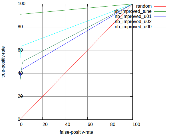
Figure 5: ROC curves of improved NB

So, for this part, I implemented Graham’s method for Bayesian Filtering, and made a little improvement for taking frequency into consideration. By the way, I think Graham should have already taken frequency into account after published the first version of his Spam Filter, or he would not have mentioned those words about Spoof in the Better (2003) post.